
 Backend Development
Python Tutorial
[Python-CVImage Segmentation : Canny Edges, Watershed, and K-Means Methods
Backend Development
Python Tutorial
[Python-CVImage Segmentation : Canny Edges, Watershed, and K-Means Methods
[Python-CVImage Segmentation : Canny Edges, Watershed, and K-Means Methods
Dec 11, 2024 am 05:33 AM
Segmentation is a fundamental technique in image analysis that allows us to divide an image into meaningful parts based on objects, shapes, or colors. It plays a pivotal role in applications such as object detection, computer vision, and even artistic image manipulation. But how can we achieve segmentation effectively? Fortunately, OpenCV (cv2) provides several user-friendly and powerful methods for segmentation.
In this tutorial, we’ll explore three popular segmentation techniques:
- Canny Edge Detection – perfect for outlining objects.
- Watershed Algorithm – great for separating overlapping regions.
- K-Means Color Segmentation – ideal for clustering similar colors in an image.
To make this tutorial engaging and practical, we’ll use satellite and aerial images from Osaka, Japan, focusing on the ancient kofun burial mounds. You can download these images and the corresponding sample notebook from the tutorial's GitHub page.
Canny Edge Detection to Contour Segmentation
Canny Edge Detection is a straightforward yet powerful method to identify edges in an image. It works by detecting areas of rapid intensity change, which are often boundaries of objects. This technique generates "thin edge" outlines by applying intensity thresholds. Let’s dive into its implementation using OpenCV.
Example: Detecting Edges in a Satellite Image
Here, we use a satellite image of Osaka, specifically a kofun burial mound, as a test case.
import cv2
import numpy as np
import matplotlib.pyplot as plt
files = sorted(glob("SAT*.png")) #Get png files
print(len(files))
img=cv2.imread(files[0])
use_image= img[0:600,700:1300]
gray = cv2.cvtColor(use_image, cv2.COLOR_BGR2GRAY)

#Stadard values
min_val = 100
max_val = 200
# Apply Canny Edge Detection
edges = cv2.Canny(gray, min_val, max_val)
#edges = cv2.Canny(gray, min_val, max_val,apertureSize=5,L2gradient = True )
False
# Show the result
plt.figure(figsize=(15, 5))
plt.subplot(131), plt.imshow(cv2.cvtColor(use_image, cv2.COLOR_BGR2RGB))
plt.title('Original Image'), plt.axis('off')
plt.subplot(132), plt.imshow(gray, cmap='gray')
plt.title('Grayscale Image'), plt.axis('off')
plt.subplot(133), plt.imshow(edges, cmap='gray')
plt.title('Canny Edges'), plt.axis('off')
plt.show()

The output edges clearly outline parts of the kofun burial mound and other regions of interest. However, some areas are missed due to the sharp thresholding. The results depend heavily on the choice of min_val and max_val, as well as the image quality.
To enhance edge detection, we can preprocess the image to spread out pixel intensities and reduce noise. This can be achieved using histogram equalization (cv2.equalizeHist()) and Gaussian blurring (cv2.GaussianBlur()).
use_image= img[0:600,700:1300]
gray = cv2.cvtColor(use_image, cv2.COLOR_BGR2GRAY)
gray_og = gray.copy()
gray = cv2.equalizeHist(gray)
gray = cv2.GaussianBlur(gray, (9, 9),1)

plt.figure(figsize=(15, 5))
plt.subplot(121), plt.imshow(gray, cmap='gray')
plt.title('Grayscale Image')
plt.subplot(122)
_= plt.hist(gray.ravel(), 256, [0,256],label="Equalized")
_ = plt.hist(gray_og.ravel(), 256, [0,256],label="Original",histtype='step')
plt.legend()
plt.title('Grayscale Histogram')
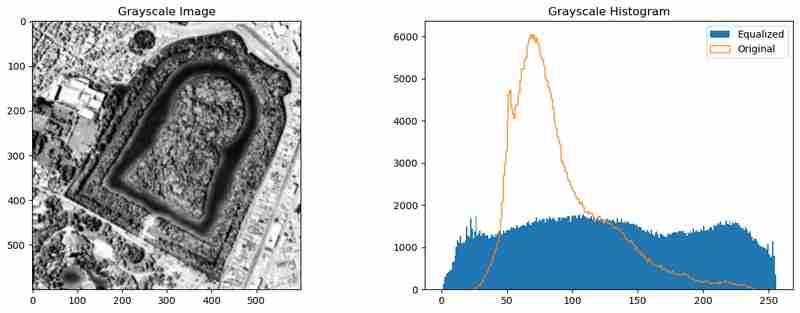
This preprocessing evens out the intensity distribution and smooths the image, which helps the Canny Edge Detection algorithm capture more meaningful edges.
Edges are useful, but they only indicate boundaries. To segment enclosed areas, we convert edges into contours and visualize them.
# Edges to contours
contours, hierarchy = cv2.findContours(edges, cv2.RETR_TREE, cv2.CHAIN_APPROX_SIMPLE)
# Calculate contour areas
areas = [cv2.contourArea(contour) for contour in contours]

# Normalize areas for the colormap
normalized_areas = np.array(areas)
if normalized_areas.max() > 0:
    normalized_areas = normalized_areas / normalized_areas.max()

# Create a colormap
cmap = plt.cm.jet

# Plot the contours with the color map
plt.figure(figsize=(10, 10))
plt.subplot(1,2,1)
plt.imshow(gray, cmap='gray', alpha=0.5)  # Display the grayscale image in the background
mask = np.zeros_like(use_image)
for contour, norm_area in zip(contours, normalized_areas):
    color = cmap(norm_area)  # Map the normalized area to a color
    color = [int(c*255) for c in color[:3]]
    cv2.drawContours(mask, [contour], -1, color,-1 )  # Draw contours on the image

plt.subplot(1,2,2)
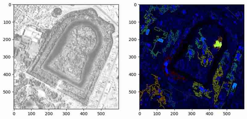
The above method highlights detected contours with colors representing their relative areas. This visualization helps verify if the contours form closed bodies or merely lines. However, in this example, many contours remain unclosed polygons. Further preprocessing or parameter tuning could address these limitations.
By combining preprocessing and contour analysis, Canny Edge Detection becomes a powerful tool for identifying object boundaries in images. However, it works best when objects are well-defined and noise is minimal. Next, we’ll explore K-Means Clustering to segment the image by color, offering a different perspective on the same data.
KMean Clustering
K-Means Clustering is a popular method in data science for grouping similar items into clusters, and it’s particularly effective for segmenting images based on color similarity. OpenCV's cv2.kmeans function simplifies this process, making it accessible for tasks like object segmentation, background removal, or visual analysis.
In this section, we will use K-Means Clustering to segment the kofun burial mound image into regions of similar colors.
To start, we apply K-Means Clustering on the RGB values of the image, treating each pixel as a data point.
import cv2
import numpy as np
import matplotlib.pyplot as plt
files = sorted(glob("SAT*.png")) #Get png files
print(len(files))
img=cv2.imread(files[0])
use_image= img[0:600,700:1300]
gray = cv2.cvtColor(use_image, cv2.COLOR_BGR2GRAY)

#Stadard values
min_val = 100
max_val = 200
# Apply Canny Edge Detection
edges = cv2.Canny(gray, min_val, max_val)
#edges = cv2.Canny(gray, min_val, max_val,apertureSize=5,L2gradient = True )
False
# Show the result
plt.figure(figsize=(15, 5))
plt.subplot(131), plt.imshow(cv2.cvtColor(use_image, cv2.COLOR_BGR2RGB))
plt.title('Original Image'), plt.axis('off')
plt.subplot(132), plt.imshow(gray, cmap='gray')
plt.title('Grayscale Image'), plt.axis('off')
plt.subplot(133), plt.imshow(edges, cmap='gray')
plt.title('Canny Edges'), plt.axis('off')
plt.show()
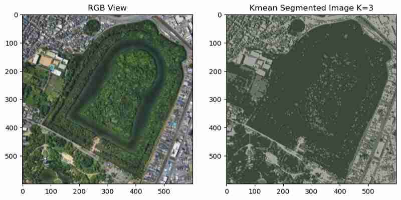
In the segmented image, the burial mound and surrounding regions are clustered into distinct colors. However, noise and small variations in color lead to fragmented clusters, which can make interpretation challenging.
To reduce noise and create smoother clusters, we can apply a median blur before running K-Means.
use_image= img[0:600,700:1300]
gray = cv2.cvtColor(use_image, cv2.COLOR_BGR2GRAY)
gray_og = gray.copy()
gray = cv2.equalizeHist(gray)
gray = cv2.GaussianBlur(gray, (9, 9),1)

plt.figure(figsize=(15, 5))
plt.subplot(121), plt.imshow(gray, cmap='gray')
plt.title('Grayscale Image')
plt.subplot(122)
_= plt.hist(gray.ravel(), 256, [0,256],label="Equalized")
_ = plt.hist(gray_og.ravel(), 256, [0,256],label="Original",histtype='step')
plt.legend()
plt.title('Grayscale Histogram')
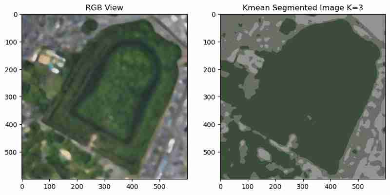
The blurred image results in smoother clusters, reducing noise and making the segmented regions more visually cohesive.
To better understand the segmentation results, we can create a color map of the unique cluster colors, using matplotlib plt.fill_between;
# Edges to contours
contours, hierarchy = cv2.findContours(edges, cv2.RETR_TREE, cv2.CHAIN_APPROX_SIMPLE)
# Calculate contour areas
areas = [cv2.contourArea(contour) for contour in contours]

# Normalize areas for the colormap
normalized_areas = np.array(areas)
if normalized_areas.max() > 0:
    normalized_areas = normalized_areas / normalized_areas.max()

# Create a colormap
cmap = plt.cm.jet

# Plot the contours with the color map
plt.figure(figsize=(10, 10))
plt.subplot(1,2,1)
plt.imshow(gray, cmap='gray', alpha=0.5)  # Display the grayscale image in the background
mask = np.zeros_like(use_image)
for contour, norm_area in zip(contours, normalized_areas):
    color = cmap(norm_area)  # Map the normalized area to a color
    color = [int(c*255) for c in color[:3]]
    cv2.drawContours(mask, [contour], -1, color,-1 )  # Draw contours on the image

plt.subplot(1,2,2)
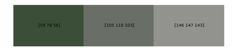
This visualization provides insight into the dominant colors in the image and their corresponding RGB values, which can be useful for further analysis. AS we could mask and select area my color code now.
The number of clusters (K) significantly impacts the results. Increasing K creates more detailed segmentation, while lower values produce broader groupings. To experiment, we can iterate over multiple K values.
import cv2
import numpy as np
import matplotlib.pyplot as plt
files = sorted(glob("SAT*.png")) #Get png files
print(len(files))
img=cv2.imread(files[0])
use_image= img[0:600,700:1300]
gray = cv2.cvtColor(use_image, cv2.COLOR_BGR2GRAY)

#Stadard values
min_val = 100
max_val = 200
# Apply Canny Edge Detection
edges = cv2.Canny(gray, min_val, max_val)
#edges = cv2.Canny(gray, min_val, max_val,apertureSize=5,L2gradient = True )
False
# Show the result
plt.figure(figsize=(15, 5))
plt.subplot(131), plt.imshow(cv2.cvtColor(use_image, cv2.COLOR_BGR2RGB))
plt.title('Original Image'), plt.axis('off')
plt.subplot(132), plt.imshow(gray, cmap='gray')
plt.title('Grayscale Image'), plt.axis('off')
plt.subplot(133), plt.imshow(edges, cmap='gray')
plt.title('Canny Edges'), plt.axis('off')
plt.show()

The clustering results for different values of K reveal a trade-off between detail and simplicity:
?Lower K values (e.g., 2-3): Broad clusters with clear distinctions, suitable for high-level segmentation.
?Higher K values (e.g., 12-15): More detailed segmentation, but at the cost of increased complexity and potential over-segmentation.
K-Means Clustering is a powerful technique for segmenting images based on color similarity. With the right preprocessing steps, it produces clear and meaningful regions. However, its performance depends on the choice of K, the quality of the input image, and the preprocessing applied. Next, we’ll explore the Watershed Algorithm, which uses topographical features to achieve precise segmentation of objects and regions.
Watershed Segmentation
The Watershed Algorithm is inspired by topographic maps, where watersheds divide drainage basins. This method treats grayscale intensity values as elevation, effectively creating "peaks" and "valleys." By identifying regions of interest, the algorithm can segment objects with precise boundaries. It’s particularly useful for separating overlapping objects, making it a great choice for complex scenarios like cell segmentation, object detection, and distinguishing densely packed features.
The first step is preprocessing the image to enhance the features, followed by applying the Watershed Algorithm.
use_image= img[0:600,700:1300]
gray = cv2.cvtColor(use_image, cv2.COLOR_BGR2GRAY)
gray_og = gray.copy()
gray = cv2.equalizeHist(gray)
gray = cv2.GaussianBlur(gray, (9, 9),1)

plt.figure(figsize=(15, 5))
plt.subplot(121), plt.imshow(gray, cmap='gray')
plt.title('Grayscale Image')
plt.subplot(122)
_= plt.hist(gray.ravel(), 256, [0,256],label="Equalized")
_ = plt.hist(gray_og.ravel(), 256, [0,256],label="Original",histtype='step')
plt.legend()
plt.title('Grayscale Histogram')
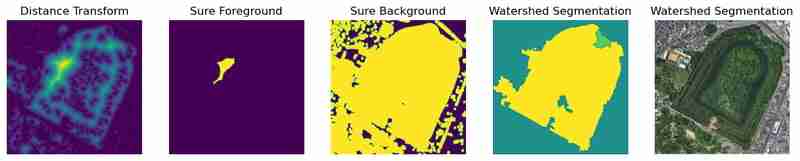
The segmented regions and boundaries can be visualized alongside intermediate processing steps.
# Edges to contours
contours, hierarchy = cv2.findContours(edges, cv2.RETR_TREE, cv2.CHAIN_APPROX_SIMPLE)
# Calculate contour areas
areas = [cv2.contourArea(contour) for contour in contours]

# Normalize areas for the colormap
normalized_areas = np.array(areas)
if normalized_areas.max() > 0:
    normalized_areas = normalized_areas / normalized_areas.max()

# Create a colormap
cmap = plt.cm.jet

# Plot the contours with the color map
plt.figure(figsize=(10, 10))
plt.subplot(1,2,1)
plt.imshow(gray, cmap='gray', alpha=0.5)  # Display the grayscale image in the background
mask = np.zeros_like(use_image)
for contour, norm_area in zip(contours, normalized_areas):
    color = cmap(norm_area)  # Map the normalized area to a color
    color = [int(c*255) for c in color[:3]]
    cv2.drawContours(mask, [contour], -1, color,-1 )  # Draw contours on the image

plt.subplot(1,2,2)
The algorithm successfully identifies distinct regions and draws clear boundaries around objects. In this example, the kofun burial mound is segmented accurately. However, the algorithm’s performance depends heavily on preprocessing steps like thresholding, noise removal, and morphological operations.
Adding advanced preprocessing, such as histogram equalization or adaptive blurring, can further enhance the results. For instance:
# Kmean color segmentation
use_image= img[0:600,700:1300]
#use_image = cv2.medianBlur(use_image, 15)


 # Reshape image for k-means
pixel_values = use_image.reshape((-1, 3)) if len(use_image.shape) == 3 else use_image.reshape((-1, 1))
pixel_values = np.float32(pixel_values)

criteria = (cv2.TERM_CRITERIA_EPS + cv2.TERM_CRITERIA_MAX_ITER, 10, 1.0)
K = 3
attempts=10
ret,label,center=cv2.kmeans(pixel_values,K,None,criteria,attempts,cv2.KMEANS_PP_CENTERS)

centers = np.uint8(center)
segmented_data = centers[label.flatten()]
segmented_image = segmented_data.reshape(use_image.shape)

plt.figure(figsize=(10, 6))
plt.subplot(1,2,1),plt.imshow(use_image[:,:,::-1])
plt.title("RGB View")
plt.subplot(1,2,2),plt.imshow(segmented_image[:,:,[2,1,0]])
plt.title(f"Kmean Segmented Image K={K}")

With these adjustments, more regions can be accurately segmented, and noise artifacts can be minimized.
The Watershed Algorithm excels in scenarios requiring precise boundary delineation and separation of overlapping objects. By leveraging preprocessing techniques, it can handle even complex images like the kofun burial mound region effectively. However, its success depends on careful parameter tuning and preprocessing.
Conclusion
Segmentation is an essential tool in image analysis, providing a pathway to isolate and understand distinct elements within an image. This tutorial demonstrated three powerful segmentation techniques—Canny Edge Detection, K-Means Clustering, and Watershed Algorithm—each tailored for specific applications. From outlining the ancient kofun burial mounds in Osaka to clustering urban landscapes and separating distinct regions, these methods highlight the versatility of OpenCV in tackling real-world challenges.
Now go and apply some of there method to an application of your choose and comment and share the results. Also if you know any other simple segmentation methods please share too
The above is the detailed content of [Python-CVImage Segmentation : Canny Edges, Watershed, and K-Means Methods. For more information, please follow other related articles on the PHP Chinese website!

Hot AI Tools

Undress AI Tool
Undress images for free

Undresser.AI Undress
AI-powered app for creating realistic nude photos

AI Clothes Remover
Online AI tool for removing clothes from photos.

Clothoff.io
AI clothes remover

Video Face Swap
Swap faces in any video effortlessly with our completely free AI face swap tool!

Hot Article
Hot Tools

Notepad++7.3.1
Easy-to-use and free code editor

SublimeText3 Chinese version
Chinese version, very easy to use

Zend Studio 13.0.1
Powerful PHP integrated development environment

Dreamweaver CS6
Visual web development tools

SublimeText3 Mac version
God-level code editing software (SublimeText3)
Hot Topics


 How does Python's unittest or pytest framework facilitate automated testing?
Jun 19, 2025 am 01:10 AM
How does Python's unittest or pytest framework facilitate automated testing?
Jun 19, 2025 am 01:10 AM
Python's unittest and pytest are two widely used testing frameworks that simplify the writing, organizing and running of automated tests. 1. Both support automatic discovery of test cases and provide a clear test structure: unittest defines tests by inheriting the TestCase class and starting with test\_; pytest is more concise, just need a function starting with test\_. 2. They all have built-in assertion support: unittest provides assertEqual, assertTrue and other methods, while pytest uses an enhanced assert statement to automatically display the failure details. 3. All have mechanisms for handling test preparation and cleaning: un
 How does Python handle mutable default arguments in functions, and why can this be problematic?
Jun 14, 2025 am 12:27 AM
How does Python handle mutable default arguments in functions, and why can this be problematic?
Jun 14, 2025 am 12:27 AM
Python's default parameters are only initialized once when defined. If mutable objects (such as lists or dictionaries) are used as default parameters, unexpected behavior may be caused. For example, when using an empty list as the default parameter, multiple calls to the function will reuse the same list instead of generating a new list each time. Problems caused by this behavior include: 1. Unexpected sharing of data between function calls; 2. The results of subsequent calls are affected by previous calls, increasing the difficulty of debugging; 3. It causes logical errors and is difficult to detect; 4. It is easy to confuse both novice and experienced developers. To avoid problems, the best practice is to set the default value to None and create a new object inside the function, such as using my_list=None instead of my_list=[] and initially in the function
 How do list, dictionary, and set comprehensions improve code readability and conciseness in Python?
Jun 14, 2025 am 12:31 AM
How do list, dictionary, and set comprehensions improve code readability and conciseness in Python?
Jun 14, 2025 am 12:31 AM
Python's list, dictionary and collection derivation improves code readability and writing efficiency through concise syntax. They are suitable for simplifying iteration and conversion operations, such as replacing multi-line loops with single-line code to implement element transformation or filtering. 1. List comprehensions such as [x2forxinrange(10)] can directly generate square sequences; 2. Dictionary comprehensions such as {x:x2forxinrange(5)} clearly express key-value mapping; 3. Conditional filtering such as [xforxinnumbersifx%2==0] makes the filtering logic more intuitive; 4. Complex conditions can also be embedded, such as combining multi-condition filtering or ternary expressions; but excessive nesting or side-effect operations should be avoided to avoid reducing maintainability. The rational use of derivation can reduce
 How can Python be integrated with other languages or systems in a microservices architecture?
Jun 14, 2025 am 12:25 AM
How can Python be integrated with other languages or systems in a microservices architecture?
Jun 14, 2025 am 12:25 AM
Python works well with other languages ??and systems in microservice architecture, the key is how each service runs independently and communicates effectively. 1. Using standard APIs and communication protocols (such as HTTP, REST, gRPC), Python builds APIs through frameworks such as Flask and FastAPI, and uses requests or httpx to call other language services; 2. Using message brokers (such as Kafka, RabbitMQ, Redis) to realize asynchronous communication, Python services can publish messages for other language consumers to process, improving system decoupling, scalability and fault tolerance; 3. Expand or embed other language runtimes (such as Jython) through C/C to achieve implementation
 How can Python be used for data analysis and manipulation with libraries like NumPy and Pandas?
Jun 19, 2025 am 01:04 AM
How can Python be used for data analysis and manipulation with libraries like NumPy and Pandas?
Jun 19, 2025 am 01:04 AM
PythonisidealfordataanalysisduetoNumPyandPandas.1)NumPyexcelsatnumericalcomputationswithfast,multi-dimensionalarraysandvectorizedoperationslikenp.sqrt().2)PandashandlesstructureddatawithSeriesandDataFrames,supportingtaskslikeloading,cleaning,filterin
 How can you implement custom iterators in Python using __iter__ and __next__?
Jun 19, 2025 am 01:12 AM
How can you implement custom iterators in Python using __iter__ and __next__?
Jun 19, 2025 am 01:12 AM
To implement a custom iterator, you need to define the __iter__ and __next__ methods in the class. ① The __iter__ method returns the iterator object itself, usually self, to be compatible with iterative environments such as for loops; ② The __next__ method controls the value of each iteration, returns the next element in the sequence, and when there are no more items, StopIteration exception should be thrown; ③ The status must be tracked correctly and the termination conditions must be set to avoid infinite loops; ④ Complex logic such as file line filtering, and pay attention to resource cleaning and memory management; ⑤ For simple logic, you can consider using the generator function yield instead, but you need to choose a suitable method based on the specific scenario.
 What are dynamic programming techniques, and how do I use them in Python?
Jun 20, 2025 am 12:57 AM
What are dynamic programming techniques, and how do I use them in Python?
Jun 20, 2025 am 12:57 AM
Dynamic programming (DP) optimizes the solution process by breaking down complex problems into simpler subproblems and storing their results to avoid repeated calculations. There are two main methods: 1. Top-down (memorization): recursively decompose the problem and use cache to store intermediate results; 2. Bottom-up (table): Iteratively build solutions from the basic situation. Suitable for scenarios where maximum/minimum values, optimal solutions or overlapping subproblems are required, such as Fibonacci sequences, backpacking problems, etc. In Python, it can be implemented through decorators or arrays, and attention should be paid to identifying recursive relationships, defining the benchmark situation, and optimizing the complexity of space.
 What are the emerging trends or future directions in the Python programming language and its ecosystem?
Jun 19, 2025 am 01:09 AM
What are the emerging trends or future directions in the Python programming language and its ecosystem?
Jun 19, 2025 am 01:09 AM
Future trends in Python include performance optimization, stronger type prompts, the rise of alternative runtimes, and the continued growth of the AI/ML field. First, CPython continues to optimize, improving performance through faster startup time, function call optimization and proposed integer operations; second, type prompts are deeply integrated into languages ??and toolchains to enhance code security and development experience; third, alternative runtimes such as PyScript and Nuitka provide new functions and performance advantages; finally, the fields of AI and data science continue to expand, and emerging libraries promote more efficient development and integration. These trends indicate that Python is constantly adapting to technological changes and maintaining its leading position.
